Georgia Tech CS 7641 - Machine Learning
Spring 2020 Final Project: Expectations Investing
Daeil Cha, Paula Gluss, Chad Hayes, Hyun Jae Park, Brett Watanabe
Motivation
Our objective is to infer stock market expectations of future company performance. In its simplest form, a stock price represents all future expectations about a company. But the stock market is ‘wrong’ many times and miscalculates future performance. Herein lies the opportunity for an investor: if he has a confident view of a company’s future performance and suspects the market’s expectations of said performance are wrong, then he has a chance to profitably trade the company’s stock. This concept is a fundamental cornerstone of investing.
As such, our goal is to systematically predict when the market will miscalculate future company performance. To our knowledge, this is a completely novel approach. We will first infer the market’s expectations using a concept called ‘expectations investing’, then compare those to actual performance. Finally, we will investigate what features are most important in causing the market to miscalculate performance. To be clear, we are not trying to predict stock returns.
Background
A Brief Primer Into Calculating Stock Prices
For context, we need to briefly discuss the calculation of stock prices. This will explain exactly what we are calculating in our model. In the most basic form, the traditional method of calculating the total value of a company is a summation of the all the future cash flows expected to be generated by the company:
Equation (i)

In reality, each future cash flow is discounted by some discount factor (the “weighted average cost of capital,” or WACC) because the future generally carries more risk. So the formula becomes this:
Equation (ii)

To derive each cash flow, for simplicity we assume some growth rate from today’s cash flow (CashFlowToday*(1+g)^i). But note that the summation goes to infinity and since no business can grow into infinite value, we have to make some adjustments. We assume the company’s cash flow will grow at some rate g1 for the nearterm (say, 10 years), then another rate g2 into perpetuity. So the formula becomes:
Equation (iii)

Note that the second term of the right side is a perpetuity. So we can rewrite the equation:
Equation (iv)

Finally, to derive the current stock price, we simply divide the company value by the company’s diluted shares outstanding. For more information about this calculation, see the following link: https://en.wikipedia.org/wiki/Discounted_cash_flow
Expectations Investing
The preceding section describes how an investor derives his own opinion of a company’s stock price. But what if we want to do the reverse? That is, the stock market’s opinion of value is simply the price a stock trades at any given time; how can we then derive the stock’s markets implicit assumptions of a company’s cash flow growth? In the framework we laid out so far, this means we want to solve for g1 (the near-term growth rate of cash flows). We will then compare the ‘market-implied’ expectation of g1 to the actual near-term growth rate realized by each company. For simplicity, we assessed the 1-year growth in cash flow.
It is straightforward to solve for the price-implied expectation of g1 by using optimization software. In equation (iv), we know the values of all the variables except for g1 and g2. Typically, g2 is assumed to be some rate lower than inflation (otherwise, the company would exceed the value of the world, which is impossible). For a deep dive into this concept of price-implied expectations of financial performance and for the inspiration behind our approach, see the following link: http://www.expectationsinvesting.com/default.shtml
Data Collection, Exploration, and Pre-Processing
Data Collection
We obtained the majority of our data from Wharton Research Data Services (WRDS), a database with a vast array of business data. For our purposes, we obtained company-specific quarterly numerical and categorical data. We also obtained macro-economic data from a variety of government websites. In total, our initial dataset consisted of 1.7 million rows of quarterly data from 1961-2020. In the future, we could consider weekly or even daily data.
Data Wrangling, Feature Engineering
The process of transforming the data was considerably extensive. We had to manually calculate the true cash flow for each company, which required knowledge of finance and accounting. We dealt with outliers by inspecting each feature’s distribution and using an intuitive understanding of what they represent. For instance, the ratio of debt to invested capital cannot be negative. We also kept data that was within 3 standard deviations of each datapoint’s respective distribution. We then scaled the numerical data with scikit-learn’s RobustScaler. We also created specific features by combining certain datapoints in different ways that we believed would be helpful for our analysis. After wrangling, our dataset consisted of 300,000 rows of 43 features in the form of time-series information from 1961 until 2020, on a quarterly basis. For a full list of each datapoint, their abbreviations, and what they represent, see the appendix.
Exploratory Data Analysis
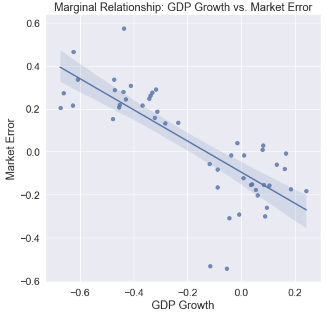
We explored the relationship between features and our label (which we call “market error”) by visualizing the marginal relationships between them. This gave us an idea of which features are important in our analysis, and how they impact the label ‘market error.’ For instance, we found a negative correlation between the growth in GDP and the market error. This suggests that the market underestimates the importance of GDP growth on future company cash flows.
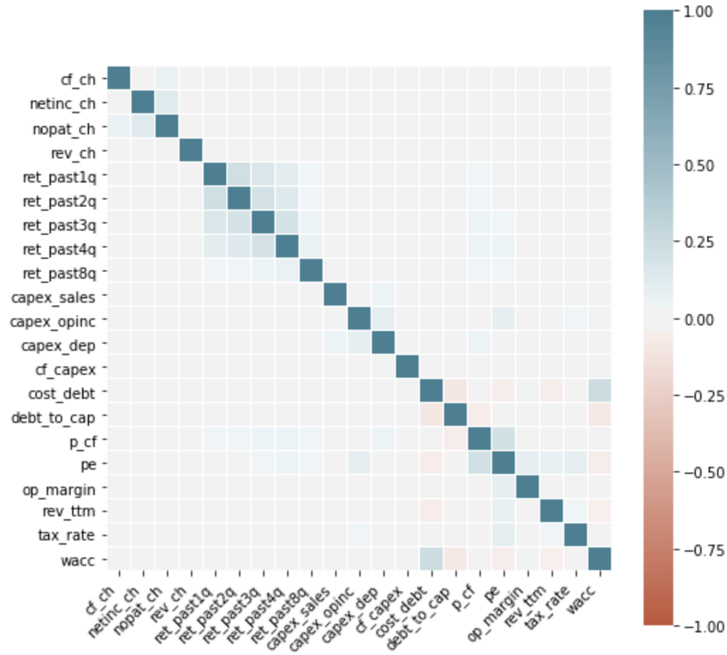
We also explored the correlation between our features. Across the entire dataset, the correlations were quite low.
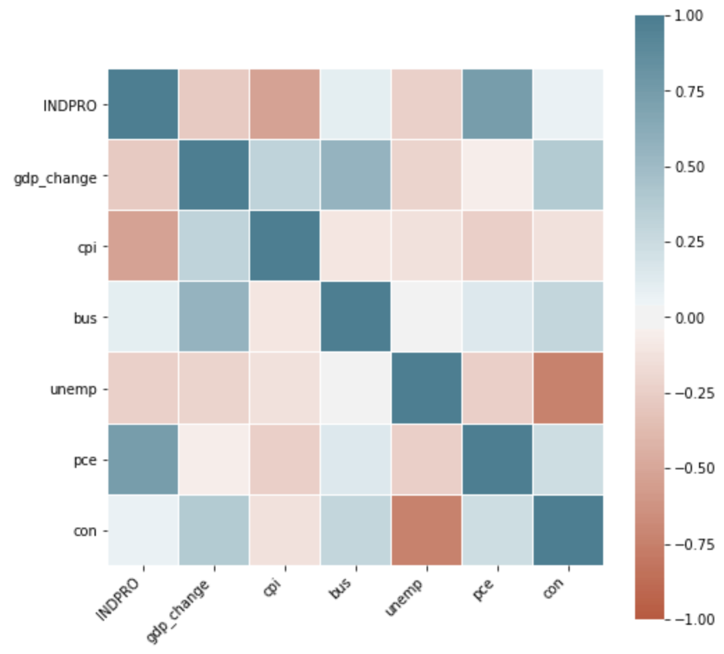
But the correlations are more pronounced for macro-economic indicators. See below:
Approach and Methods
Our primary approach is to use classification methods to determine when the market will either overestimate or underestimate growth in a company’s cash flow. To our knowledge, our approach is novel for two reasons:
- Market expectations of financial performance have never been systematically analyzed.
- Machine learning has never been applied to predicting market expectations of financial performance.
We should first note a particular observation about the data. We created a new label for classification; if the market error of future growth (g1 - g1_actual) was positive, we applied a 1 as the classification label; otherwise we applied a 0. Before modeling, we noticed that the percent of 1’s in the data was 57%. This sets a baseline for performance, and any classifier we train would be considered effective if its accuracy for identifying 1’s is greater than 57%.
Supervised Learning
Below we outline the results of 9 different classification methods on our data. We found that a Random Forest classifier worked best, and it saw an accuracy, precision, recall, and F1 score of 75.98%, 76.07%, 86.22%, and 80.83%, respectively. We consider these are strong results especially in relation to the baseline of 57%. We should note that investors are focused on precision (maximizing the percent of profitable trades) over recall (capturing all the profitable trades possible). For a number of reasons, a fundamental principle of investing is to avoid losses whenever possible.
| Supervised Model | Accuracy | Precision | Recall | F1 |
|---|---|---|---|---|
| Logistic Regression | 60.21 | 66.8 | 64.12 | 65.43 |
| K-Nearest Neighbors | 57.92 | 63.05 | 68.61 | 65.67 |
| Random Forest | 75.98 | 76.07 | 86.22 | 80.83 |
| Gaussian Naive Bayes | 59.06 | 59.47 | 95.18 | 73.2 |
| Decision Tree | 65.44 | 70.86 | 69.92 | 70.38 |
| Linear SVM | 59.7 | 66.45 | 63.4 | 64.89 |
| Non-Linear SVM | 57.86 | 63.68 | 65.78 | 64.71 |
| Feed-Forward Network | 65.7 | 64.87 | 90.75 | 75.65 |
| LSTM Network | 66.48 | 67.56 | 82.58 | 74.32 |
From the random forest model we were able to obtain feature importance. The top 5 most influential features were in the following order:
- Price to cash flow [Label 1 Mean : 0.0028 / Label 0 Mean : 0.8096]
- Change in cash flow [Label 1 Mean : 0.0337 / Label 0 Mean : -0.1008]
- Price to trailing net income [Label 1 Mean : -0.143 / Label 0 Mean : 0.3316]
- Change in revenue [Label 1 Mean : 1.1042 / Label 0 Mean : 1.6879]
- Net operating margin [Label 1 Mean : -0.1479 / Label 0 Mean : 0.2035]
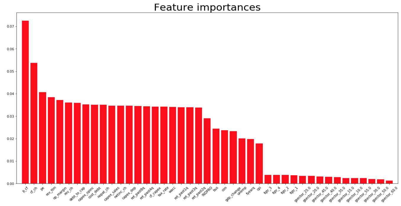
This result aligned with our lasso regression model results as shown below.
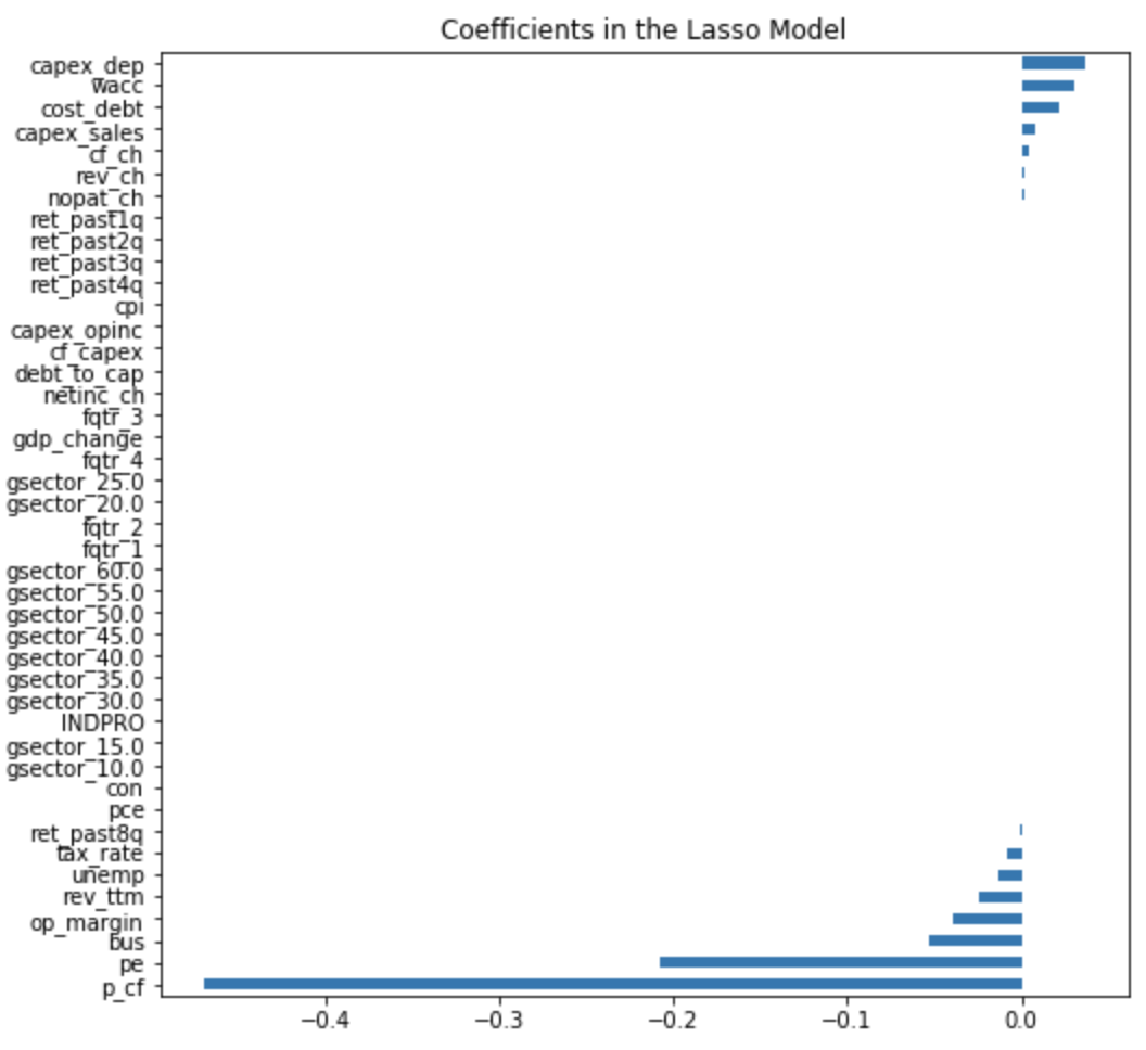
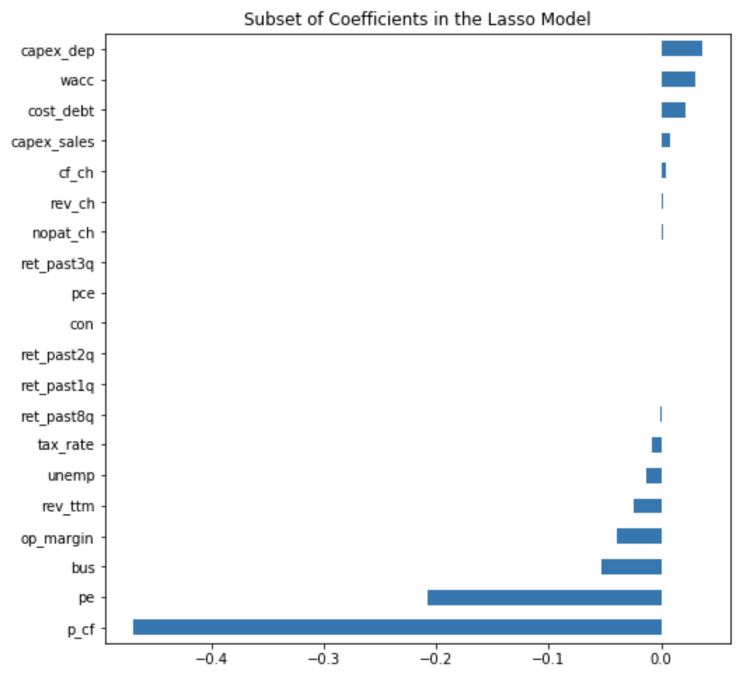
We simply omitted those features with 0 values for coefficients, which showed that 15 features were important. The five most important features in the random forest model were captured in the Lasso regression as well.
Unsupervised Learning
We also considered unsupervised learning methods: specifically, clustering algorithms. Using only the features in our dataset, we found the following results.
| K-Means Number of Clusters | Silhouette Score | Davies-Bouldin Score |
|---|---|---|
| 5 | 0.7777 | 0.1594 |
| 6 | 0.7869 | 0.2239 |
| 7 | 0.808 | 0.202 |
| 8 | 0.8162 | 0.2129 |
| 9 | 0.8221 | 0.2046 |
| 10 | 0.775 | 0.2375 |
| 11 | 0.7716 | 0.2293 |
| 12 | 0.7626 | 0.2597 |
This suggests that stocks can be clustered using our features since the Silhouette scores are relatively high and the Davies-Bouldin scores are low. We see that the best results are generated when k is 9 clusters.
Now that we have these clusters, what can we do in context with our experiment? Do the clusters say anything helpful about how much the market miscalculates future business performance? We inspected the mean and variance of our label (the market error of the future) for 9 clusters, and we did not find conclusive evidence that our clustering approach has predictive power. The mean of the labels were between 57-61%, which is not impressive given that baseline accuracy is around 57%. Also, the standard deviation of the label was high (between 48-49%). See the results below (note: ‘LABEL’ which was used for supervised learning was not included during clustering, but the mean and standard deviation of ‘LABEL’ were calculated afterwards to see if certain stocks clustered together frequently differed from market expectations).
| Cluster Number (9 Clusters) |
Data Points in Cluster |
Mean of Cluster (LABEL) |
Std. Dev of Cluster (LABEL) |
|---|---|---|---|
| 0 | 23,569 | 0.5966 | 0.4906 |
| 1 | 2 | 0.5 | 0.5 |
| 2 | 1 | 0 | 0 |
| 3 | 23,323 | 0.5692 | 0.4952 |
| 4 | 19,455 | 0.6116 | 0.4874 |
| 5 | 82,321 | 0.6002 | 0.4898 |
| 6 | 7,790 | 0.5801 | 0.4935 |
| 7 | 122,919 | 0.5745 | 0.4944 |
| 8 | 5,244 | 0.5896 | 0.4919 |
Additionally, we attempted other clustering algorithms (e.g. DBSCAN), but silhouette / Davies-Bouldin scores were significantly worse than using K-means with 9 clusters.
Results and Discussion
As we noted, the market overestimated future performance 57% of the time from 1961 through the beginning of 2020. This by itself is potentially profound, as it suggests stock investors tend to be overly optimistic about future business performance. For decades, behavioral economists have attempted to characterize the biases of investors through controlled studies (see prospect theory), but our analysis shows real-world systematic errors made by professional investors. A study of the time series of the market’s errors would be another experiment to consider in the future; that is, it would be interesting to investigate the nature of the market’s errors during different economic regimes like stock bubbles or recessions.
Regarding our dataset, we should note that it was necessary to retain outliers in some of the stock market data (particularly the market’s expectation of growth) because the market does indeed exhibit extreme, erratic behavior at times, and this behavior is precisely what we wanted to capture.
Regarding our machine learning analysis, we believe the random forest classifier performed the best because deep decision trees can capture complex structure that other algorithms might miss. The random forest then averages many trees—a powerful tool for handling high variance and noise, which our dataset exhibits (as is the nature of financial data). By contrast, linear regression is weak to outliers; again, which our data has. Further, support vector machines (SVM) does not handle high dimensionality very well, so we are not surprised by its relatively weaker results.
According to our results from the random forest and logistic regression model, we will discuss the intuition behind the predictive power of the features with the most extreme values.
-
Highest Coefficients (causes market to overestimate future performance)
-
Capital expenditures to depreciation: This is the ratio of capital investments a company makes over a given time to the depreciation of its existing investments. While a company that seeks growth must invest in its assets faster than its assets depreciate, it appears that investors overestimate the importance of this variable.
-
WACC and Cost of debt: WACC is the “weighted average cost of capital,” or the amount that a company’s capital (debt and equity) cost per year. It could make sense that investors do not sufficiently account for the cost of capital when forecasting future growth, and therefore overestimate growth when that cost is high. But this could also simply be a function of our approach, and of where g1 and WACC sit in the calculation of stock prices: numerator and denominator, respectively.
-
Capital expenditures to sales: This is the ratio of a company’s capital investments to its sales. While capital expenditures are necessary for growth, a ratio that is too high could suggest a deteriorating financial position, or that the company is unable to achieve growth without spending significantly more; perhaps investors are overly relying on this metric.
-
-
Lowest Coefficients (causes market to underestimate future performance)
-
Price to cash flow: This is a company’s stock price in relation to its cash flow per share. This metric has the strongest predictive power of any of the other features. There is a reason that the financial community has the mantra: “Cash is king.” Despite whatever accounting methods are used to show profitability, cash does not lie. As such, cash generation and company value are inextricably linked. A high price to cash flow ratio for a stock suggests the stock is priced too high, and investors should be skeptical. But it appears that investors become too skeptical and tend to underestimate growth in stocks with high price to cash flow ratios. If an investor simply avoids a stock with a high price to cash flow ratio, he might miss a trading opportunity. This is an interesting result that suggests that a theoretical understanding of finance and stocks is not enough to profitably invest; one must also understand game theory and the behavior of others.
-
Price to earnings: This is a company’s stock price to its earnings per share. The intuition behind this metric’s predictive power is similar to that of price to cash flow. But as we mentioned: earnings can be manipulated whereas cash is king.
-
We uncovered some interesting, counterintuitive results from our analysis. First, we found that it is possible to reliably predict the market’s error in estimating the future. Second, the features that cause these market errors are somewhat counterintuitive from a textbook finance perspective. We also learned that processing financial data can be exceptionally difficult, not only because there is significant variance and noise in the numbers, but also because the decisions to handle outliers or other issues require an intuitive understanding of each datapoint and of the inter-relationships between all datapoints. Regardless, we believe our work has non-trivial implications in the realm of behavioral economics and investing, and opens possibilities for new research.
Contributions
Proposal: All
Data Collection: Daeil
Data Wrangling: All
Exploratory Data Analysis: Hyun Jae
Variable Selection: Paula
Visualization: Paula, Hyun Jae
Modeling: Michael (Chad)
Analysis and Conclusion: Brett and all
Github and Writeup: All
References and Sources
https://data.oecd.org/leadind/business-confidence-index-bci.htm
https://data.oecd.org/leadind/consumer-confidence-index-cci.htm
https://data.oecd.org/price/inflation-forecast.htm
https://en.wikipedia.org/wiki/Discounted_cash_flow
https://fred.stlouisfed.org/series/INDPRO
https://fred.stlouisfed.org/series/PCEC96
https://fred.stlouisfed.org/series/GDP
https://wrds-web.wharton.upenn.edu/wrds/process/wrds.cfm
https://www.bls.gov/charts/employment-situation/civilian-unemployment-rate.htm
https://www.eia.gov/dnav/pet/hist/LeafHandler.ashx?n=pet&s=f000000__3&f=m
http://www.expectationsinvesting.com/default.shtml
https://en.wikipedia.org/wiki/Prospect_theory
Appendix
Notes on Data Wrangling & Feature Engineering
Nearly all of our data was temporal, and we needed to calculate changes in certain metrics over fixed intervals. As such, we ensured that all the dates in our dataset were contiguous. We noted that there were some duplicate rows, and some jumps in data (this can happen when a stock de-lists from an exchange and re-lists later). We ensured that our calculations accounted for these issues.
To generate the ‘market error’ label for our project (market expectations of cash flow growth versus actual growth), we required quarterly cash flows for each company. This is not so simple as downloading cash flow figures from a database, because those figures can include extraordinary one-time items that are not reflective of real business performance, and because quarterly numbers of cash flow are not reliably available (at least in the database we used). So we downloaded all the elements required to calculate cash flow:
Equation (v)
Free Cash Flow to Firm = Net Operating Profit After Tax + (Depreciation & Amortization) - Capital Expenditures - Change in Net Working Capital
We also needed to manually calculate Net Operating Profit After Tax (NOPAT), which reflects business profit:
Equation (vi)
NOPAT = (Net Income + Taxes Paid + Interest Expenses Paid + Non-Operating Gains/Losses) * (1 - Tax Rate)
Note that NOPAT adds back taxes paid, interest paid, and non-operating losses. This is done to adjust for items that can fluctuate widely and do not necessarily relate to core business operations.
Once we calculated free cash flow for each company at each date, we then calculated actual growth in cash flow (4 quarters), which is g1_actual. We then derived market expectation (g1) by taking each date’s stock price, using equation (iv), and solving for g1 for every stock at every date by using optimization software. We assumed that g2 is 0.015 for all companies; this is typically set at a rate below inflation because otherwise the company’s value would exceed that of the world, which is impossible.
Notes on the Label
Our label is the absolute difference between the market’s expectation of growth in cash flow, versus realized growth in cash flow (G1 - G1_ACTUAL). Intuitively, this represents how much the market miscalculates a company’s future growth.
Numerical Features (Company Specific)
CAPEX_SALES - Capital expenditures to last 12 months of sales (capxy / rev_ttm). A high ratio suggests a deteriorating financial position.
CAPEX_OPINC - Capital expenditures to yearly operating cash flow (capxy / nopat_ttm)
CAPEX_DEP - Capital expenditures to yearly depreciation and amortization (capxy / (4 * dpq))
CF_CAPEX - Cash flow to capital expenditures (cf_ttm / capxy). This measures a company’s ability to acquire long-term assets using free cash flow. A higher ratio suggests sufficient capital to fund operations.
CF_CH - Year-on-year change in trailing 12 months cash flow
COST_DEBT - cost of debt
DEBT_TO_CAP - Debt to invested capital (dlttq / icaptq)
DEBT_TO_MCAP - Debt to market capital (dlttq / mkvaltq)
MKVALTQ - Market value
NETINC_CH - Year-on-year change in trailing 12 months net income
NOPAT_CH - Year-on-year change in trailing 12 months net operating profit after tax
P_CF - Price to trailing 12 months of free cash flow to firm (prccq / (cf_ttm / cshfdq))
PE - Price to trailing 12 months of net income (prccq / (netinc_ttm / cshfdq))
OP_MARGIN - Net operating margin (nopat_ttm / rev_ttm)
REV_CH - Year-on-year change in trailing 12 months revenue
RET_PAST1Q - Stock return trailing 1 quarter
RET_PAST2Q - Stock return trailing 2 quarters
RET_PAST3Q - Stock return trailing 3 quarters
RET_PAST4Q - Stock return trailing 4 quarters
RET_PAST8Q - Stock return trailing 8 quarters
TAX_RATE - Tax rate
WACC - Weighted average cost of capital
Categorical Features (Company Specific)
FQTR - Calendar quarter during which the data was reported
GGROUP - GIC Groups
GIND - GIC Industries
GSECTOR - GIC Sectors
GSUBIND - GIC Sub-Industries
NAICS - North American Industry Classification Code
SIC - Standard Industry Classification Code
Numerical Features (Macro-Economic Data)
INDPRO - Industrial Production
GDP_CHANGE - Change in annualized GDP
CPI - Inflation (measured by Consumer Price Index)
BUS - Business confidence index
UNEMP - Unemployment rate
PCE - Personal Consumption
CON - Consumer confidence index